Assignment of Part 2: CO2 Disposal in a Depleted Gas Reservoir: An Impact Assessment Study
Prof. Chris Spiers
High Pressure and Temperature Laboratory (HPT Lab), Department of Earth Sciences, UU
CO2 Disposal in a Depleted Gas Reservoir: An Impact Assessment Study
1. The Problem to be tackled
In this assignment, you will consider the environmental impact of CO2 disposal in a depleted (exhausted) natural gas reservoir. As discussed in the lectures, this means of CO2 disposal may prove to be one of the most important uses of underground space in the coming 50 years, as an interim strategy for reducing CO2 emissions into the atmosphere. You will analyze a generic (fictitious) case in order to gain insight into the “side effects” of CO2 disposal underground, the problems involved and how to deal with them.
2. Essential Background
Utilization of underground space always leads to some kind of disturbance of the geological and/or surface environments, which must be evaluated. Typically, the underground force- (i.e. stress-), position- (or deformation-), temperature- and groundwater flow fields are affected. If we pump CO2 into a porous reservoir rock unit, how will that and the surrounding rock respond? These questions fall within the discipline of “Rock Mechanics”, a branch of Rock Physics. Before tackling your assignment, you must therefore be introduced to the basics of rock mechanics and the physical properties of reservoir rocks. You must also be introduced to the properties of compressible gaseous fluids, specifically the pressure-volume-temperature (P-V-T) behaviour or equation of state of CO2.
3. Introduction to rock mechanics
Rock mechanics deals with the way that rock materials respond to applied forces (stress) under given conditions of temperature and overburden or confining pressure (depth). The response is measured in terms of shape change (distortion, deformation, strain) or shape change rate (deformation rate or strain rate). Let’s consider the main concepts below.
3.1. What is rock mechanics?
- Rock mechanics deals with the reponse of the rock (compaction, deformation, fracture, flow (strain or strain rate) to applied forces (stress).
- "Stress - strain (rate) relations" describe shape change produced !!
- "Failure criteria" describe the stress conditions (loading) at which rock breaks !
3.1.1. Stress and strain defined for uniaxial loading (cylindrical sample)
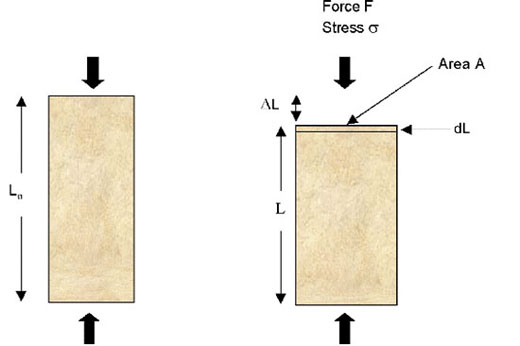
Figure 1. Uniaxial loading
- Axial stress σ = F/A (N/m2 or Pa)
- Axial strain e = (Lo - L) / Lo = ΔL/ Lo
- Strain increment dε=dL / L
- Strain rate
dε/dt = (1/L)dL/dt (s-1)
- Compressive stress and strain can be taken as positive or negative !!!!
3.1.2. Simple shear loading
- Shear stress τ = F/A (Pa)
- Shear strain γ= tanθ = Δ L/L0
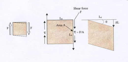
Figure 2. Simple shear loading
3.1.3. Hydrostatic (isotropic) loading
- Hydrostatic (isotropic) pressure P = F/A (Pa)
- Volumetric strain ev = ΔV/V0
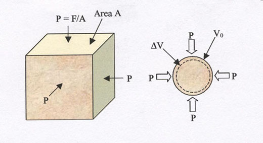
Figure 3. Hydrostatic loading
3.2. Classes of mechanical behaviour
3.2.1. Elastic
- Recoverable deformation
- Time-independent
- Linear: σ proportional to e
- Slope = Elastic modulus (Young's modulus E, Shear mod G, or Bulk mod K)
- Strains small (< 0.5%)
- Mechanism = bond stretching
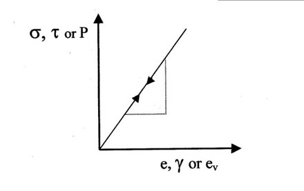
Figure 4. Strain versus stress
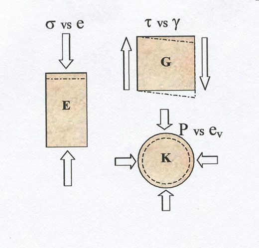
Figure 5. Stress, strain and corresponding modulus
3.2.2. Brittle
- Permanent fracture / fault
- Strength loss / drop
- Time-independent (largely)
- Seismic / acoustic emission !!!
- Mechanism = crack nucleation / propagation / coalescence
Figure 6. Beyond critial strength: rupture
3.2.3. Ductile
- Permanent cohesive deformation or flow
- Like plasticine or a soft metal
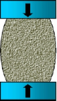
Figure 7. Flow upon stress load
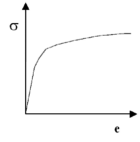
Figure 8. (much) more flow with just marginally increased stress
- May be time (rate) independent:
- e = f(σ) only, at fixed T. Examples: Metals at room T, wet clays
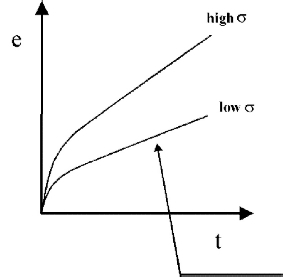
Figure 9. Time dependence
- May be time (rate) dependent:
- e = f(σ,t) at fixed T. Examples: rocksalt in crust, silly putty
- Steady state creep
 (cf. viscous flow of liquids)
- Various atomic scale mechanisms!! You'll learn about these in the 3rd year.
3.3. Some important variables in the crust
- Stress and temperature
- "Overburden pressure" or "lithostatic pressure" (also called "confining pressure")
- - pressure due to overburden
- - P = ρgh (h = depth)
- - Units: Pa (that is N/m2). N.B. 1 atmosphere is ca. 1 bar = 105 Pa = 0.1 MPa!!
- - dP /dh = ρg is ca. 20 - 25 MPa/km
- Pore fluid pressure Pf
- - Counteracts P
- - Pf = (0.4 ® 1.0) Pf typically ca. 0.5 P
- Effective (confining) pressure Pe = P - Pf
- - Controls brittle / frictional behaviour
- - Changes in Pe produce elastic response too!
3.4. Stress state in 3-D bodies
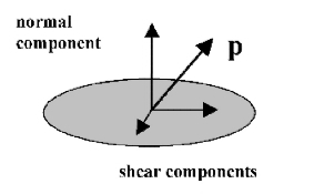
Figure 10. Stress vector p
- Stress transmitted across any plane in a 3-D body can be described by a vector p (force vector per unit area)
- p varies with plane orientation in body
- State of stress in 3-D body is a second order tensor σij:
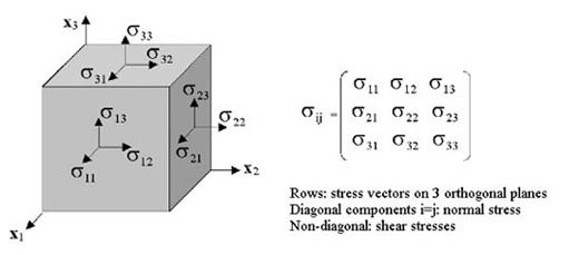
Figure 11. Stress tensor
3.5. Principal stresses
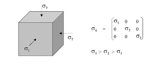
Figure 12. Principal stresses σij
- Eigen vectors / values of σijyield principal stresses σi:
- Three such directions can always be found (no shear stresseson orthogonal planes)
- Principal stresses form the simplest way to define stressstate (shear components zero) !!
3.5.1. In the upper crust:
- principal stresses ~ vertical and horizontal

(no shear stress at Earth surface) - vertical stress is approximately equivalent to the lithostatic or overburden pressure P
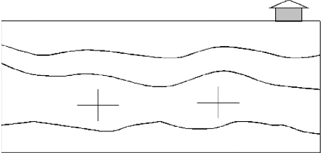
Figure 13. Principal stresses in the upper crust
3.5.2. Stress in 2-D
- Principal stresses:
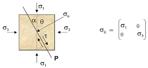
Figure 14. Principal stress relationships
- Stresses on any plane P depend on the orientation of that plane (i.e. on θ)
- σn = 1/2 (σ1+σ3)+ 1/2 (σ1-σ3)cos2θ
- τ = 1/2 (σ1-σ3)sin2θ
- Try to prove this for yourselves sometime!
- Mohr circle representation
The above equation link τ,σn and θ via the "Mohr circle"

Figure 15. Mohr circle
3.5.3. Strain in 3-D
- Strain is also a second order tensor (many forms)
- Most easily expressible in terms of principal strains
- Examples:
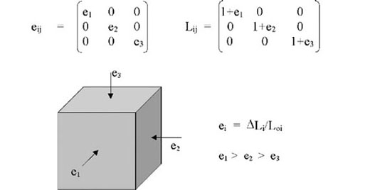
Figure 16. Strain tensor
- Ratio of principal strains (e.g. ei) determines shape change:
- When strains are small(e < 0.1%) and material is isotropic, principal strains are parallel to principal stresses !!!!!
Figure 17. Small strain and isotropic material
3.6. Modes of brittle failure or fracture
N.B. Brittle failure involves σ1 and σ3 only (2-D problem) !!
3.6.1. Extensional Failure
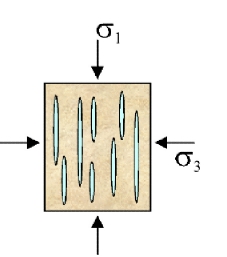
Figure 18. Extensional failure
- Occurs in wet rock when Pf ® (σ3+T0) (hydrofracture)
- To is tensile strength of the rock
- Stability criterion: Pf < (σ3+T0)
- Weak seismic emission
3.6.2. Shear Failure
Figure 19. Shear failure
- Occurs when σ1 > σ3 >> 0 (compressive)
- Note conjugate fault planes
- Strong(er) seismic emission (BANG!!)
- Shear failure occurs when Coulomb criterion is satisfied:
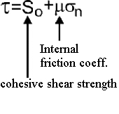
Figure 20. Coulomb criterion

Figure 21. Shear failure depicted in stress diagram
So conjugate fractures typically form at α approximately 30o and θ approximately 60o to σ1 !!!!!
- In Mohr diagram:
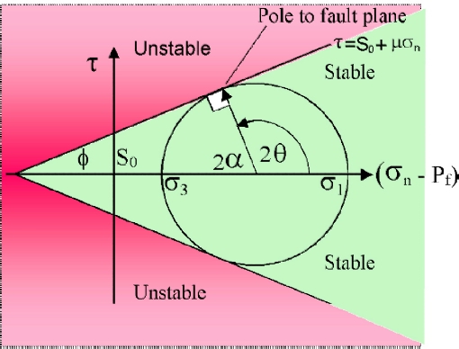
Figure 22. Mohr diagram
tanΦ = μ, tan2θ = -1/μ, μ approximately 0.5, θ approximately 60o
3.6.3. Alternative form of Coulomb criterion:
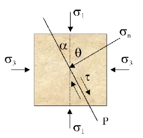
Figure 23. Shear failure depicted in stress diagram
Substituting the equations for stresses on plane P i.e.,
σn = 1/2 (σ1+σ3) + 1/2 (σ1-σ3)cos2θ and τ = 1/2 (σ1 - σ3)sin2θ,
into the Coulomb criterion τ = S0 + μσn gives the alternative failure criterion
(σ1/σ3)= Q{2(So - Pf)/σ3+q}
which in turn gives the stability criterion
(σ1/σ3)< Q{2(So - Pf)/σ3+q}
where Q = sin2θ /(1 + cos2θ) and q = (1 - cos2θ)/sin2θ
4. Properties of reservoir rocks
We will now consider the rock mechanical properties of porous reservoir rocks, such as sandstones, as relevant to the extraction or injection of fluids (oil, water or gasses) on human time scales. As discussed in the lectures, fluid pumping operations will change the pore fluid pressure (Pf) within the rock and therefore the state of stress in the reservoir formation. For example, a decrease of pore pressure by oil or gas exploitation increases the effective overburden pressure (Pe = P - Pf), or vertical stress, felt by the rock. This will lead to vertical compaction of the reservoir by elastic processes, or by permanent deformation (by grain crushing or pore collapse) if the vertical stress becomes high enough. An increase in pore pressure will generally lead to vertical expansion by elastic processes. Horizontal displacements are negligible because the surrounding rock prevents lateral expansion of the reservoir.
The response of a reservoir rock to changes in pore pressure at constant vertical stress σ1 can thus be pictured as follows:
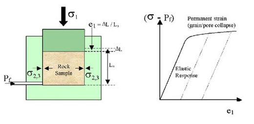
Figure 24. Reservoir rock loading and response
The full 3-D elastic response is described by the poroelastic equation (Wang 2000). This is written in terms of the 3 principal strains (e1, e2, e3) and stresses (σ1, σ2, σ3) as
ei = a.σi- b(σ1+σ2+&sigma3)+c.Pf
For any change (ΔX) in stress or pore pressure, it gives the changes in the principal strains as
Δei = a.Δσi- b(Δσ1+Δσ2+Δσ3)+c.ΔPf
Here
a = 1/(2G) b = (3K - 2G)/(18KG) c = (1/Kg - 1/K)/3 and i = 1, 2, 3
where G is the shear modulus of the rock,
K is its bulk modulus and
Kg is the bulk modulus of the mineral grains making up the rock.
Note that if the effective vertical stress σ1-Pf) reaches a sufficiently high level (the "yield stress"), permanent deformation (compaction) occurs by grain crushing and/or pore collapse. Under appropriate conditions, shear fractures may tend to form. Over a long period of time, creep effects may also become important in compaction mode.
5. Properties of CO2 - equation of state
The pressure-volume-temperature (P-V-T) relations, or equations of state, for fluids (liquids, vapours, gasses) such as water and CO2 are of major importance in the Earth Sciences for understanding both the chemical and physical roles of these fluids in the lithosphere and hydrosphere. These relations are also crucial for calculating how much CO2 can be disposed of in reservoir rock formations.
For typical in situ reservoir conditions (P > 20 MPa = 200 bar, T > 40 oC), the phase diagram for CO2 shows that it will be in the supercritical fluid/vapour state (critical point ~30 oC !!!!!).
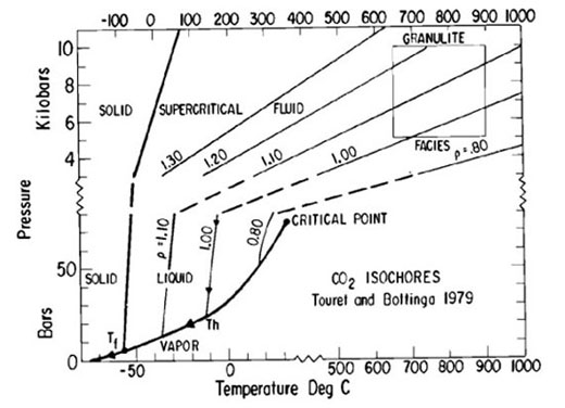
Figure 25. Phase diagram for CO2 showing the P-T fields in which CO2 is solid, liquid, gas and supercritical fluid/vapour. Contours show density of the liquid and supercritical fluid phases relative to water at NTP.
As you will (hopefully) remember from high-school, the P-V-T relation for an ideal gas is written
PV= nRT or P = RT/v
where n is number of moles of gas, R is the universal gas constant (8.314 J/mol/K), v is molar volume and T is absolute temperature (Kelvin K). This gives a poor approximation for the P-V-T behaviour CO2 under reservoir conditions, or indeed for any gaseous fluid under geological conditions. The two-term Van der Waals modification, which accounts for both attractive and repulsive forces between gas molecules, written
P = {RT / (v - b)} - a/v2
(where a and b are constants), is an improvement. A further improvement, based on a more detailed analysis of molecular interaction forces, is provided by the Redlich-Kwong equation (Redlich & Kwong, 1949):
P = {RT/(v-b)} - {a / [v(v +b)]}. T-1/2
This can be still further improved by the inclusion of additional interaction forces in the RT term (Carnahan & Starling, 1972) and by recognizing that a = a(P,T) (Kerrick & Jacobs, 1981). The result obtained is known as a Modified Redlich Kwong equation (MRK equation) (Kerrick & Jacobs, 1981). The MRK equation given by Kerrick & Jacobs (1981) takes the form
P = RT(S)/{v(v-y)3} - {a(P,T) / [v(v +b)]}.T-1/2
where y = b/4v
S = (1 + y + y2 - y3)
a = c + (d / v) + (e / v2)
This MRK equation is widely used in describing the properties of both water and CO2 under Earth conditions.
For CO2, Kerrick & Jacobs (1981) presented the following, experimentally derived values of b, c, d and e, which can be used as input for calculating its P-V-T behaviour under geological conditions:
b = 58
c = [28.31 + (0.12 x T) - (8.8 x 10⁻³ x T2)]x 106
d = [9380 - (8.53 x T) + (1.2 x 10⁻³ x T2)]x 106
e = [-368654 + (716 x T) + (0.15 x T2)] x 106
An Excel program ("CO2-Calc-2") is provided with this assignment to allow you to calculate v as a function of the temperature and pressure of CO2 using these data in conjunction with the above MRK equation. Note that only two input variables are needed by the programme, namely P + T. All of the necessary data on CO2 are contained in the programme.
6. The Assignment Itself
It is 2012 and you are working for a government geosciences and environmental watchdog agency. Your boss puts you on the following job.
An oil company exploiting the natural gas reservoir (porous sandstone) shown in the schematic profile below has extracted gas for a ten year period, reducing the reservoir pore pressure from 35 MPa to a value now close to zero. The reservoir is therefore completely exhausted. The gas production operation has led to reservoir compaction and to accompanying surface subsidence, reaching 25 cm above the thickest part of the reservoir. The company is now proposing to dispose of CO2 produced by electricity generating industry by injecting it into the reservoir on a commercial basis. In so doing, the company also hopes to restore the original surface topography, thereby minimizing any possible long-term environmental effects.
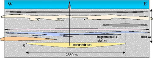
Figure 26. Schematic geological cross section showing the exhausted gas reservoir into which CO2 is to be injected (profile not to scale). The section passes through the thickest part of the reservoir.
6.1. The challenge
Before the oil company carries out their planned operation, your agency (YOU !) must conduct an independent evaluation of reservoir capacity and the possible environmental impact of the scheme. The following questions must be answered:
- What mass of CO2 can be disposed of in the reservoir if the original pore pressure of 35 MPa is to be reached?
- Will re-establishment of the original pore pressure by injecting CO2 return the reservoir top to its original position, thereby restoring the surface topography to the initial elevation?
- Is returning the pore pressure to its original value likely to induce seismicity (i.e. fracturing within the reservoir)?
- If the original topography cannot be restored by injecting CO2 to the initial pore pressure, what CO2 pressure would be needed? Would increasing the pore pressure to this value be likely to cause seismicity, and would there be any additional risks associated with going to the higher pressure?
- What is the impact of restoring the pore pressure to its original value of 35 MPa likely to be at the surface?
6.2. The data needed
To answer the above questions, you have asked colleagues in the rock mechanics and geophysics sections of your agency to supply you with data on the reservoir dimensions, on the in-situ conditions and on the reservoir rock properties. These data are given in the following table. Note that compressive stresses and displacements are taken as positive.
(immediately before CO2 injection) | Form: Plano-convex (~sinusoidal base) Depth to top = 1800 m Max. Thickness = 79 m Total rock volume = 1.3 x 10⁸ m3 Average porosity (void/total volume) = 12.5 % Water volume per unit rock volume = 5 % Average density of overburden = 2280 kg/m3 Vertical stress σ1 is ca. overburden pressure (constant) E-W stress σ3 is ca. 23.0 MPa N-S stress σ2 is ca. 27.9 MPa Pore pressure = 0.0 MPa Reservoir temperature = 59 oC (332 K) |
| Shear modulus of rock G = 2.20 GPa Bulk modulus of rock K = 7.20 GPa Bulk modulus of rock grains Kg = 28.7 GPa | |
| τ = S0+ μσn S0 = 2.5 MPa μ = 0.5 Pf = σ3 + To To = 1.5 MPa | |
| Use Modified Redlich-Kwong (MRK) equation given earlier plus spreadsheat program "CO2-Calc-2" |
The Excel programs that you need are here.
Program 1: ReservoirCalc-Blank.
Program 2: CO2-Calc-2-Blank.
6.3. Your brief
Your brief is to carry out the steps listed below. Write down your answers/results by hand as you go, using them at the end as a basis for writing a professional report.
Exercise 1A. Use the data given on reservoir form and in-situ conditions to calculate the pore volume available for CO2 disposal within the reservoir.
Exercise 1B. Go on to calculate the number of moles n and the mass of CO2 that can be stored in the reservoir at the target pore pressure Pf of 35 MPa, assuming negligible changes in the reservoir volume during injection and negligible uptake of CO2 by water in the rock pores. Tip: First make a rough estimate of n using the ideal gas law PV = nRT. Then use the MRK equation for CO2 given earlier and incorporated in the Excel program "CO2-Calc-2". Note that the CO2 will be in supercritical fluid/vapour form in the reservoir rock! Read the text about the MRK equation before using it!
Exercise 2A. Write out the poroelastic equation for changes in the state of strain of reservoir rock, taking i = 1, 2 and 3.
Exercise 2B. Assuming that changes in pore pressure (ΔPf) caused by pumping CO2 into the reservoir lead to vertical displacements only (no horizontal displacements), what will the change in the horizontal strains (Δe2 and Δe3) be at any point in the reservoir during injection?
Exercise 2C. Assuming the overburden pressure at mid depth in the reservoir (1839.5 m) to be roughly constant and equal to the average vertical stress (σ1) acting throughout the rock unit, write down approximate expressions for &sigma1 and Δσ1 during CO2 injection.
Exercise 2D. Now use the poroelastic equation (your answer to part A) to derive algebraic equations relating the vertical strain response of the reservoir rock (Δe1) to changes in gas pressure (ΔPf).
Exercise 2E. Similiarly, show how the horizontal stresses (Δσ2, Δσ3 and σ2, σ3) depend upon ΔPf (tip: denote the initial values of the horizontal principal stresses as σ2initial and σ3initial).
Exercise 3. Use your results from Part 2 to qualitatively answer the following questions:
- will the reservoir sandstone compact or expand vertically when CO2 is injected ?
- what will happen to the horizontal stresses in the reservoir during injection?
Exercise 4. The poroelastic equations you have derived are incorporated into the Excel program "ReservoirCalc". Use this program to plot how the vertical strain and horizontal stresses in the reservoir vary as the injected CO2 pressure is increased to 40 MPa (just beyondthe target value of 35 MPa). N.B. The program will also display the Coulomb failure criterion and the hydrofracture criterion for the reservoir, assuming that the maximum principal stress (σ1) remains vertical and that the minimum principal stress (σ3) remains horizontal E-W.
Exercise 5. Use your results and worksheets 3 and 4 of "ReservoirCalc" to answer the following:
- Are the qualitative effects of increasing Pf that you inferred from your analytical results in Part 3 confirmed by the plots produced using "ReservoirCalc". (If not, go back to 3 and check!).
- Will the reservoir recover its original shape when the target CO2 pressure of 35 MPa (i.e. the original gas pressure) is reached? Explain your answer.
- What will be the final conditions in the reservoir when the target pressure is reached?
- Is induced seismicity likely to occur during the injection of CO2 to the target pressure of 35 MPa? Explain your answer.
- What would the impact at the surface be, if the surface environment is a) an intertidal flat, or b) a major city (choose a. or b. according to your own interest).
- Would there be any advantage in increasing the target pressure beyond 35 MPa? Explain your opinion!
Exercise 6. Finally, if you select this assignment for the full report, write a professional report using the title and structure suggested in the table below. Use the PAR and IMRAD-C approaches to writing. Use the standard IMRAD-C format (Introduction - Methods - Results - Discussion - Conclusions) embedded in sections 1, 2, 3-5, 6, and 7 respectively. If you don't use this format, your score will be seriously degraded!
| Title | Impact of CO2 disposal in adepleted gas reservoir |
| Executive Summary | 2/3-page summary for "guys in ties" - thisis essential in any technical report that might go to top bosses or politicians |
| 1. Introduction | State: |
| 2. Methods and data | Outline calculation methods, give equations used, give data used |
| 3. Storage capacity | - Present your results on this topic |
| 4. Reservoir response to CO2 injection | - Give response in terms of strain, displacement and stresses vs. Pf |
| 5. Seismicity | Present your results on whether or not seismicity is likely to be induced by CO2 injection to the target pressure |
| 6. Discussion: Environmental Impact | Write up a discussion/evaluation of the impact you expect for your chosen surface environment. Mention possible effects of exceeding 35 MPa CO2 pressure |
| 7. Summary/conclusions | Summarize your main findings / inferences for the scientific and technical readership |
| References | List any references to the literature in the standard way. This is used in my reference list!!! |
Table showing you how to structure your report in a professional way. Note the use of the standard IMRAD-C format (Intro - Method - Results - Discussion - Conclusions) embedded in sections 1, 2, 3-5, 6 and 7 respectively. The conclusions serve as a technical summary. The Executive Summary is for "bosses" - use the PAR format for this (Abstract format of Problem - Action - Result).
Rereferences
Carnahan, N.F. and Starling, K.E., 1972. Intermolecular repulsions and the equation of state for fluids. Am. Inst. Chem. Eng., 18, 1184-1189.
Kerrick, D.M. and Jacobs, G.K., 1981. A modified Redlich-Kwong equation for H2O, CO2, and H2O-CO2 mixtures at elevated pressures and temperatures. Am. J. Sci., 281, 735-767.
Redlich, O. and Kwong, J.N.S., 1949. An equation of state. Fugacities of gaseous solutions. Chem. Rev., 44, 233-244.
Touret, J. and Bottinga, Y., 1979. Equation d'etat pour le CO2; application aux inclusions carboniques. Bull. Mineralogie, 102, 577-583.
Wang, H.F., 2000. Theory of linear poroelastiscity with
applications to geomechanics and hydrology, Princeton University Press, 340 pp.