Assignment of Part 1: System Earth and the Challenge of Sustainable Development
POPULATION PROJECTIONS
1. Introduction
Population projections are useful for a variety of purposes, commonly as a basis for planning and policy making, but also, for example, in assessing future food requirements and resulting land degradation, and the threat to forests from our ever growing population concentrations. We will use the population projections to make estimates about future consumption of the Earth’s non-renewable resources, such as fossil fuels, gold, iron ore, and rare earths. Doing that will enable us to make predictions on when these non-renewable resources become depleted.
The demographic model in Spectrum, known as DemProj (Stover & Kirmeyer, 1997), is a computer program for making population projections for countries or regions. The program requires information on the number of people by age and sex in the base year, as well as current year data and future assumptions about the total fertility rate (TFR), the age distribution of fertility, life expectancy at birth by sex, the most appropriate life table, and the magnitude and pattern of international migration. This information is used to project the size of the future population by age and sex up to the year of 2100.
2. Background: Projection Model Parameters
DemProj projects future populations on the basis of model patterns for fertility (TFR and age distribution of fertility) and mortality (life expectancy at birth and age-specific mortality). These will be discussed in the following sections.
2.1. Fertility
The TFR is the number of live births a woman would have if she survived to age 50 and had children according to the prevailing pattern of childbearing at each age group. An assumption about the future TFR is required for most population projections. Projected fertility is affected by certain age characteristics, for example, appropriate fertility rates need to be assigned by age group, as those groups vary in size, which contributes to the size of the population being projected to the next period. In addition, some implications of population projections follow from the age of the mothers as they bear children. In DemProj, the age distribution of fertility is entered as the percentage of lifetime fertility that occurs in five-year groups 15-19, 20-24, 25-29, 30-34, 35-39, 40-44, and 45-49. Base year fertility rates are usually available from national fertility surveys. From these, the required percentage distribution of age-specific fertility rates can be obtained.
To convert TFR to age-specific fertility rates, population projections use i) the United Nations Models tables (Table 1), which are based on statistics, or ii) the Coale-Trussell Relational Fertility Model. The Coale-Trussell model, first introduced in 1974 (Coale and Trussell, 1974, 1978; United Nations, 1983), is the most widely accepted model of the age composition of fertility.
Table 1. United Nations tables of the age distribution of fertility (click to download excel file)
The Coale-Trussell model decomposes age-specific fertility rates into three factors corresponding to basic fertility determinants:
- natural fertility: hypothetical fertility that might exist in the absence of birth control, if all women were in sexual unions during their entire reproductive spans.
- birth control: deliberate control over childbearing by way of contraception and/or abortion.
- cohabitation (consensual or marital): time spent by women within sexual unions, with time in unions being shortened due to premarital sexual abstinence, spousal separation, or dissolution of the union.
The model formalized the relationship between age-specific fertility and its determinants in a simplified form. It assumes that:
- natural fertility within unions is proportional to a certain age schedule that is approximated the same for different populations;
- the intensity of birth control is also proportional to a standard age schedule; and
- the age shape of the proportion currently in unions is similar to the age-specific proportion of ever-married individuals in a female population.
According to the model any set of age-specific fertility rates, f x is given by
 (1)
(1)
where G x is the model proportion who ever married, M is a scale factor reflecting the average impact of marriage/union interruption, n x is the standard schedule for natural fertility, m the model parameter of birth control, and v x is a standard pattern of birth control impact on fertility. G x is formalized, based on a standard density function, which in turn takes two parameters:
- the singulate mean age of marriage (SMAM), which is the arithmetic mean age at first marriage; and
- the initial nuptial age (a 0 ), which is the age at which a significant number of sexual unions start.
In DemProj, the Coale-Trussell model is simplified. It is assumed that in a projection period, the fertility change which occurs would affect primarily the stopping patterns for higher-order births, the birth-spacing pattern, and that the marriage pattern and the pattern of spacing of lower-order births are not be altered. The model demonstrates a relationship between the projected age-specific fertility rates (f a) and the reference fertility rates (f 0,a ) as
 (2)
(2)
Here v a is the Coale-trussell standard age specific schedule of fertility control (Table 2). The total fertility rate (TFR) is then represented as:
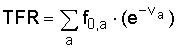 (3)
(3)
Table 2. Coale-Trussell fertility control schedule (click to download excel file)
2.2. Mortality
Mortality is described in DemProj through two assumptions: life expectancy at birth by sex, and a model life table of age-specific mortality rates.
2.2.1. Life expectancy at birth
Life expectancy at birth is the average number of years that a cohort of people would live, subject to the prevailing age-specific mortality rates. Life expectancy at birth can be calculated from vital statistics on deaths if reporting is complete, however, life expectancy usually has to be estimated from large-scale surveys. Any population projection requires assumptions about future levels of life expectancy. The most used is the United Nations modelschedule of changes in life expectancy. This schedule assumes that life expectancy at birth, for both males and females, increases by 2.0 to 2.5 years over each five-year period when life expectancy is less than 60 and then increases at a slower rate at higher levels. Table 3 shows the working model used in the United Nations population projections.
2.2.2. Age-specific mortality
The mortality input in DemProj, life expectancy at birth, indicates overall mortality in a population. But DemProj also needs the pattern of mortality in order to produce mortality rates by age group. These patterns are given by two sets of model life tables: the Coale-Demeny model tables which apply to Europe and other industrialized regions, and the United Nations tables for developing countries (very specific regions). An example pattern (Coale-Demeny West model table) is given in Figure 1. The most appropriate model life table will be the one that most closely matches the crude death rate (CDR) and infant mortality rate (IMR) for that country or region.
2.3. International migration
International migration refers to the number of migrants moving into or out of the area for which the population projection is being prepared. Usually, international migration can be ignored without a significant effect on the population projection for countries. For specific regions or cities however, migration can be very important.
2.4. Current population: Urban and Rural
DemProj can be used to make urban and rural population projections along with the national projection. We will not use this option of DemProj, therefore we will not go into how this can be accomplished.
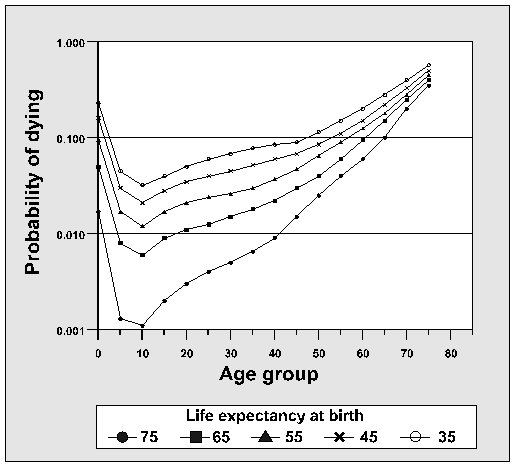
Figure 1. Coale-Demeny West model life table.
3. Background: Methodology
DemProj calculations are based on the standard cohort component projection modified to produce a single-year projection.
3.1. Calculating the base population by single ages
The first step is to separate the population by five-year age groups into single years of age. This is achieved through the use of the Beers formulas (Beers, 1945; see appendix A ).
3.2. Survival ratios
Survival ratios are the proportion of the population of a particular age that survives to the next age in the next year. The life tables used in DemProj provide single-year survival ratios from birth to age one, age one to two, two to three, three to four, and four to five. Beyond age five the tables provide five-year survival ratios. These five-year survival ratios are converted to single-year survival ratios by taking the fifth root of the five-year survival ratio.
3.3. Deaths
Deaths for a particular age and sex are calculated asfollows:
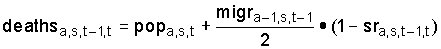 (4)
(4)
where deaths a,s,t-1,t is deaths occurring as people age from age group a-1 at time t-1 to age a at time t, pop a,s,t is the population of age group a and sex s at time t, migr a-1,s,t-1 is the net number of migrants of age group a-1 and sex s at time t-1, and sr is the survival ratio or proportion of age group a-1 and sex s at time t-1 that survives to age group a at time t.
3.4. Population size
The population of most age groups is calculated as the number of people one year younger one year ago, plus the net migration during the year, minus the number of deaths:
 (5)
(5)
For the last age group, the population also includes those who were in the last age group one year ago and survive to the present year:
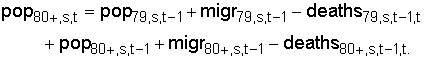 (6)
(6)
The population under one year of age is calculated as the number of births during the year that survive to the end of the year plus the net migrants:
 (7)
(7)
3.5. Births
The number of births in a year is calculated from the number of women of reproductive age, the TFR and the age distribution of fertility.
 (8)
(8)
where births a,t is the number of births to women at age a, TFR t is the total fertility rate at time t, and ASFP a,t is the proportion of lifetime fertility that takes place at age a. Total births are found by summing births to women in all the reproductive ages
 (9)
(9)
Births by sex are calculated from total births and the sex ratio at birth.
 (10)
(10)
4. Background: Program Tutorial
Population projections that you will need have been made already for you. If you like to play with the program DemProj yourself, it can be downloaded from
http://www.policyproject.com/software.cfm?page=Software&ID=Spectrum
After installation you can make your population projections (if you wish of course, in Windows Vista the editor is hung after certain operations. You can quit the program via the task manager and redo your projection). Following is a step by step manual to make a population projection using DemProj.
- Open Spectrum
- Click New projection
- Fill in a name at Projection title
- Set First Year to 2015
- Set Final Year to 2100 (further is not possible)
- Fill in a Projection file name by clicking on the button 'projection file name', a folder where the file is stored appears.
- Click Easyproj and select the country or region
- Click OK (the projection is being calculated with the optimal parameters for that area)
- Click Display, Demography (DemProj), Population,Total population
- You can play with projection plotting parameters via the dialog box. By using alt-PrintScreen you capture the active window and can put it in another program.
- If you wish to change projection input parameters: Click Edit, Demography (DemProj)
- Click Demographic data
- Change data to the First year population table
- Change data to the Life expectancy table
- Change data to the Total fertility rate table
- Change the most appropriate Model life table
- Neglect International migration and fill in the Sex ratio at birth
- Click OK and then Close
- Click Display, Demography (DemProj), Population,Total population
- the changed projection appears and can be saved under a different name (preferably).
5. References
- Beers, H.S., 1945. Six-term formula for routine actuarial interpolation, The Record of the American Institute of Actuaries, vol. 34 Part I, 59-60.
- Coale, A.J. and Trussell, T.J., 1974. Model fertility schedules: Variations in the age structure of childbearing in human populations, Population Index, vol. 44, 185-258.
- Coale, A.J. and Trussell, T.J., 1978. Technical note: Finding the two parameters that specify a model schedule of marital fertility, Population Index, vol. 44, 203-213.
- Stover, J. and Kirmeyer, S., 1997. DemProj: A computer program for making population projections, The Futures Group International and Research Triangle Institute, http://www.policyproject.com/software.cfm?page=Software&ID=Spectrum
- United Nations, 1983. Manual X: Indirect techniques for demographic estimation, New York, United Nations.
Exercises
Exercise 1: a) What could be a reason why the population models for the various countries and regions that have been provided to you are so different? b) Fit two straight lines through the graph of the world population projection that describe the essence of the curve in a plausible way. Use those lines in the next exercises. It may be clear that you are using 'eye ball statistics' to (gu)es(s)timate the lines. Nonetheless some lines are more reasonable than others. What would be a strategy to arrive at an optimal estimate?
Exercise 2: Making use of the result of exercise 1 and the data given in Appendix C , determine when we run out of oil (incorporate EUR oil), natural gas and coal at present (2013) per head consumption rates. (Use Windows Excel to do this exercise.)
Exercise 3: Same as above, determine when gold, iron ore, and rare earth elements will be depleted (2014 consumption rates, calculate on a per capita basis). Determine two values, one based on reserve and one on reserve base. In this exercise, take production rate = consumption rate. (Resource data given in Appendix C .)
Exercise 4: a) Taking the present (2014) per capita energy consumption, when will all fossil fuels be depleted? b) Repeat this exercise, but now assume that the whole world will achieve a life style closer to the present-day American style of living (2014 American energy consumption) over a period of 50 years. In the scenario calculation take a 3% per year increase in consumption for the non-USA population. (Resource data given in Appendix C .) c) We now turn our attention to the rare earth elements. If consumption increases 100 times when are they depleted? (Resource data given in Appendix C .)
Exercise 5: Figure 2 demonstrates that the predicted lifetimes for various reserves have changed considerably from 1970 to 2005. As example, according to the 1970 predictions metals like lead, gold, mercury, zinc, silver, tin and copper should have been depleted before the year 2000, clearly this is not the case. Considering Figure 2 and the exercises you just performed yourself, answer the following questions.
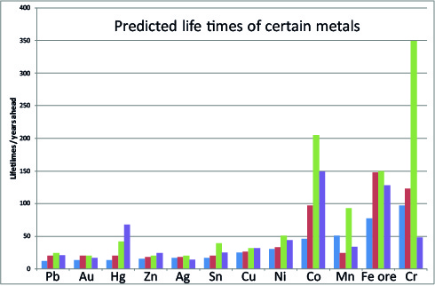
Figure 2. Lifetimes of some reserves as predicted in 1970 (blue), in 1992 (red), in 1996 (green), and in 2005 (purple).
Question 1: What could be plausible reasons for widely varying trends in the predicted population growth behaviour?
Question 2: Why are the reserve lifetime predictions over the years so different from the ones you did yourself?
Question 3: Are predictions on reserve lifetimes useful? If no, why not? If yes, why so?
Question 4: What is the role of Earth sciences in lifetime predictions of reserves?
Question 5: What is the role of economy in lifetime predictions of reserves?
Question 6: What is the role of environmentalism in lifetime prediction of reserves?
Answer the questions concisely and implement these aspects in the discussion of your report if you choose this topic to write the full report. Success with writing it! (upon selection)